Introduction to geodata research
This site gives an overview of the advantages and drawbacks of geodata, how research currently uses geodata and how georeferencing works for administrative and survey data.
1. Why use geodata?
Understanding how local contexts shape life chances requires more than knowing which municipality or county a person lives in. Geodata allow us to move beyond administrative borders and study social and economic environments with much greater precision.
Traditional analyses rely on administrative units such as municipalities or counties. This approach has clear limitations.
- First, data must be available at exactly the same administrative level, which is not always the case.
- Second, administrative boundaries change over time (for example through territorial reforms in Germany), making longitudinal comparisons difficult.
More importantly, administrative units implicitly assume that everyone within them is exposed to the same context. In reality, this is rarely true. A household located near the border of a county may be more strongly influenced by opportunities, labour markets, or institutions in the neighbouring region than by those in its own county.
Geocoded residential data allow us to measure spatial exposure more accurately, for example by calculating distances, defining flexible neighbourhood radii, or constructing grid-based spatial units. In this way, geodata help align theoretical concepts of “local context” with empirically meaningful spatial measures.
Example: administrative boundaries vs. exact locations
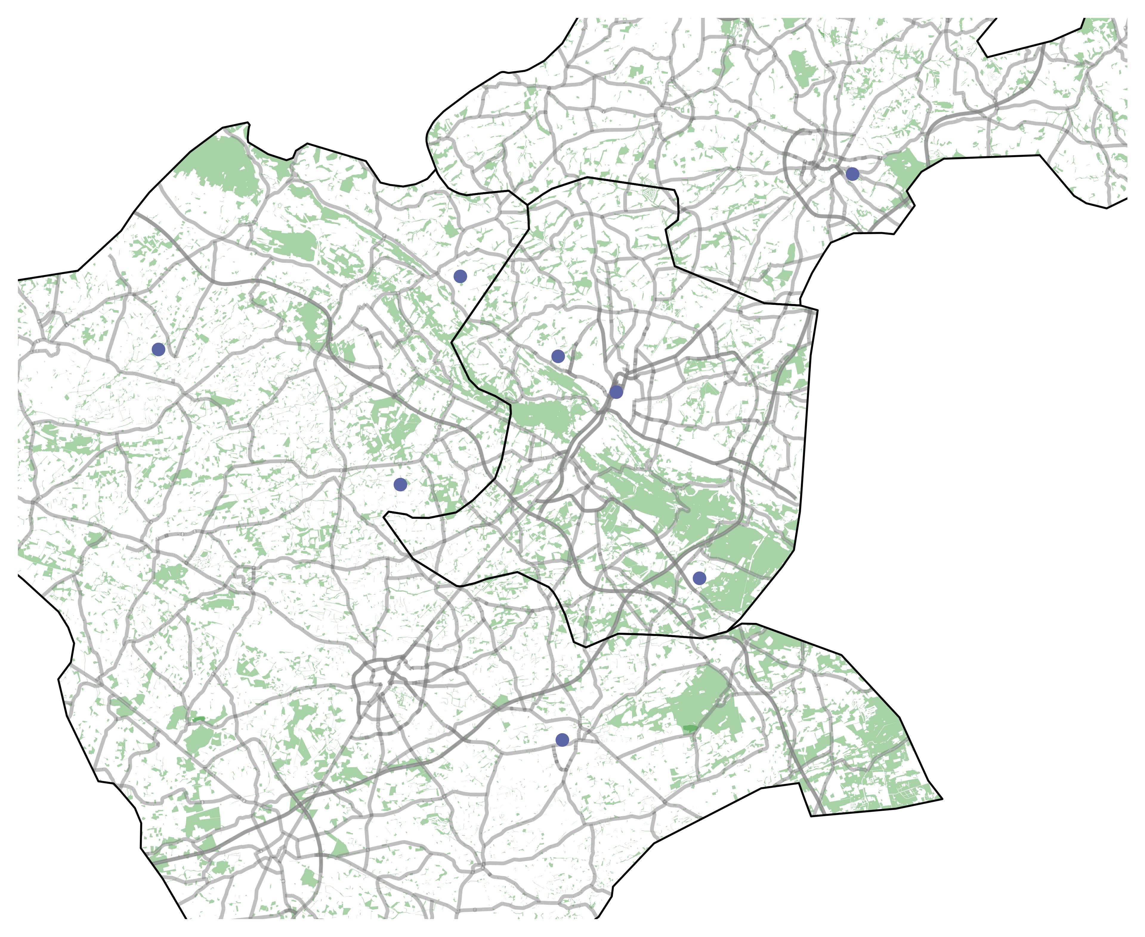
In the example map, the black lines depict administrative units (here counties, German “Landkreise”). Many data sets already contain information on county-aggregated statistics (such as the mean unemployment rate or population size). However, these administrative units often change over time (e.g. “Gebietsstandsreformen” in Germany), complicating panel analyses with such indicators. The blue dots represent individuals located at different locations in a county. Some are in the middle of a county, whereas others are closer to county boundaries. Especially for the latter, characteristics or the labour market structure of the adjacent county may be more relevant.
2. How geodata are used in research
Georeferenced data open up a wide range of empirical strategies:
- Studying regional shocks: Identifying how local events or policy changes affect individuals depending on their exact location.
- Example: Ahlfeldt et al. (2015) exploit the fall of the Berlin Wall to investigate agglomeration and dispersion forces.
- See also Dube, Lester and Reich (2010), who estimate effects across state borders using pairs of contiguous counties.
- Distance-based measures: Calculating proximity to institutions, infrastructure, or labour markets
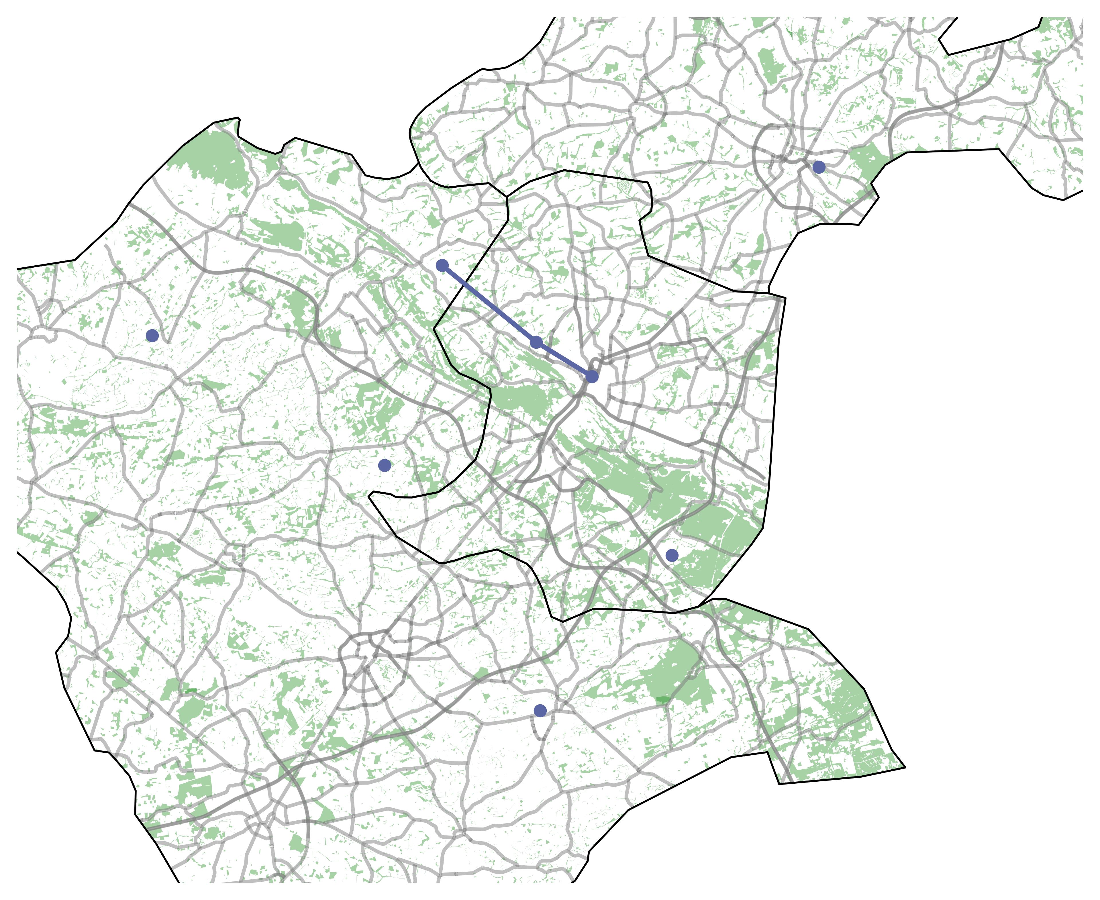
- Figure 2, panel (a) provides a visual example of “as-the-crow-flies” distance calculations. Three dots are connected via two blue lines. The dot in the middle shows a shorter distance to the eastern dot.
- Scientific paper: Currie et al. (2010) show that the distance to fast food restaurants in miles correlates with the individual’s weight gain.
- Figure 2, panel (a) provides a visual example of “as-the-crow-flies” distance calculations. Three dots are connected via two blue lines. The dot in the middle shows a shorter distance to the eastern dot.
- Radius-based approaches: Defining neighbourhoods using buffers around residential locations (“egohoods”).
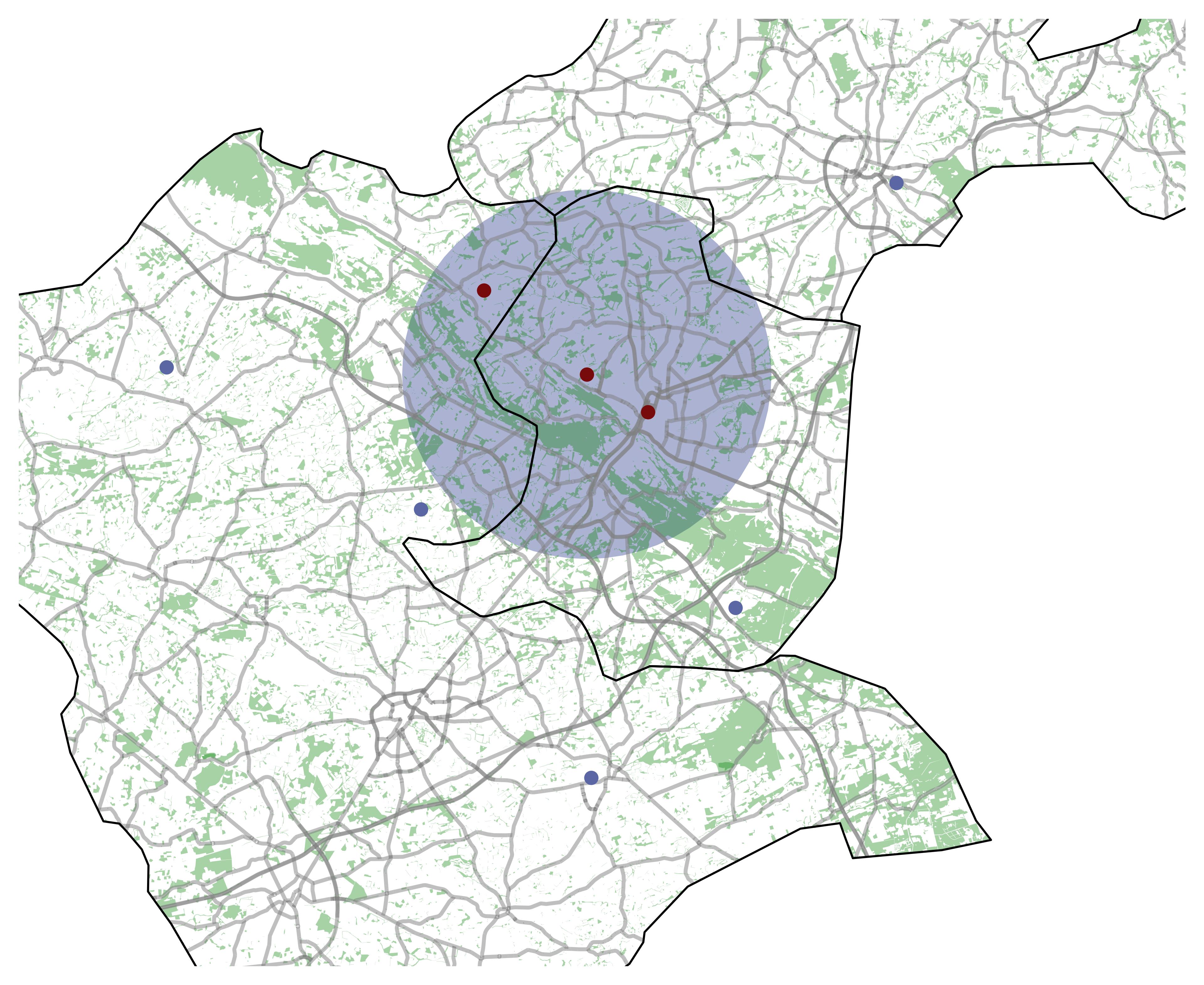
- Figure 2, panel (b) provides a visual example of a radius calculation. The radius-buffer shows the same distance to every radius boundary and covers two additional dots.
- Scientific paper: Laurence and Goebel (2025) employ egohoods with varying radii to measure segregation and interethnic contact probabilities.
- Grid-based measures: Defining contexts using grid cells rather than administrative borders
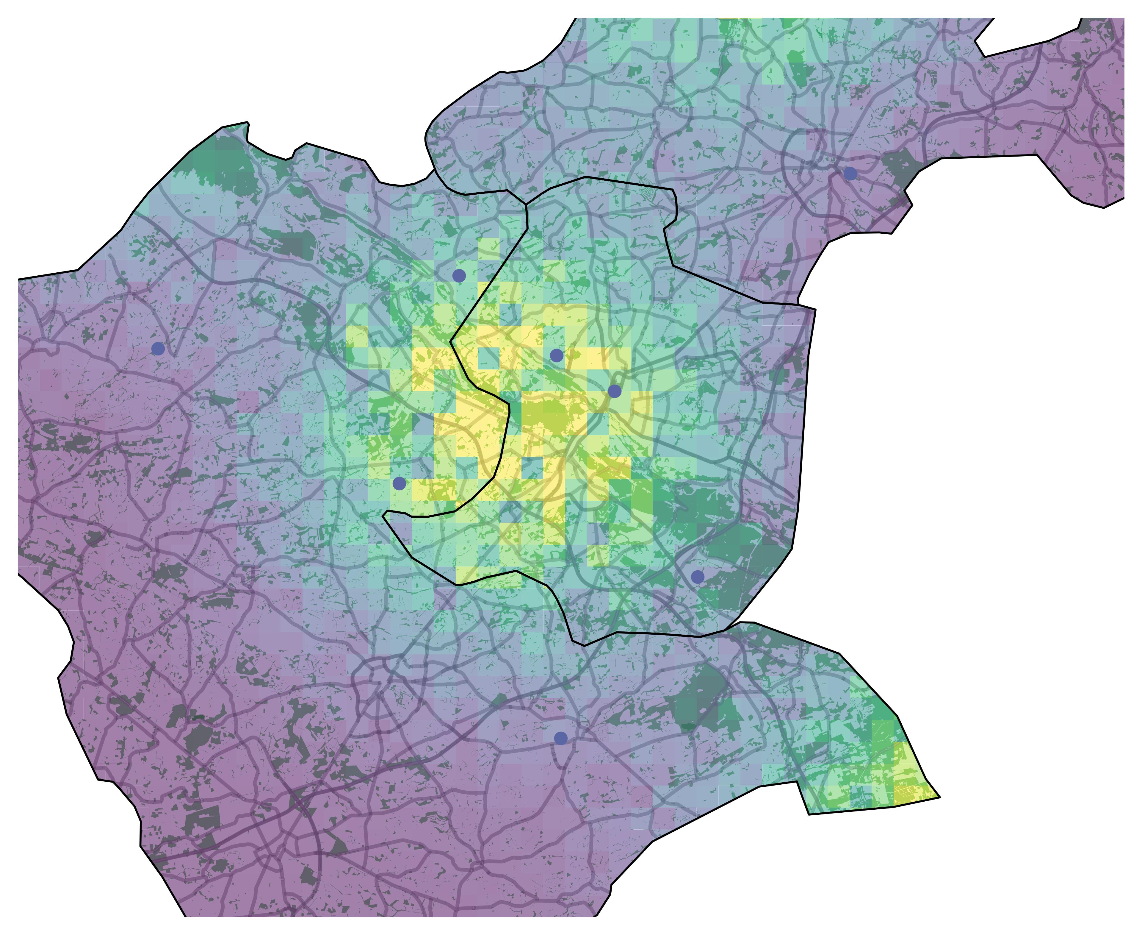
- Figure 2, panel (c) provides a visual example of grids in adding an additional grid-layer to the map. While the grid colors follow a random data generating process, the grid structure shows that grid-based aggregated information can be more detailed than county-aggregated information.
- Scientific paper: Ostermann et al. (2022) provide extensive map material based on 1x1km grid cells for all German cities with more than 100,000 inhabitants based on administrative data.
- Density-based methods: Identifying spatial concentrations using kernel density estimation or clustering algorithms.
- Scientific paper: Ostermann (2026) uses a hierarchical density-based clustering algorithm (HDBSCAN) to delineate neighbourhoods in German metropolises.
- Linking external data: Combining observational or survey data with environmental or infrastructural datasets.
- Spatial sampling strategies: Designing samples based on geographic criteria.
- Scientific paper: Roth et al. (2026) use cluster sampling where all individuals from the selected districts (“Auswahlbezirke”) are interviewed to investigate whether migrants pay higher rents for comparable housing.
Illustration of different spatial operationalisations
Geodata substantially improve how we measure and analyse local opportunity structures. Instead of relying on fixed administrative categories, they allow researchers to define spatial contexts in ways that better reflect lived environments and theoretical concepts.
What geodata cannot capture
Despite these advantages, geocoded residential addresses are not a perfect measure of spatial exposure.
They identify where a building is located, but not the exact position of a dwelling within the building. For example, in studies of environmental exposure, it may matter whether an apartment faces a busy street or a quiet courtyard.
In addition, residential addresses do not reveal how much time individuals actually spend at home. Daily mobility, commuting, and activity spaces remain unobserved. Geodata therefore provide a highly useful, though still partial, approximation of people’s spatial environments.
3. Geocoding administrative labour market data
One source of georeferenced data in Germany comes from the administrative records of the Institute for Employment Research (IAB). These data contain detailed employment biographies of individuals who are:
- employed,
- receiving benefits,
- searching for a job,
- participating in firm-based vocational training, or
- enrolled in active labour market policy programmes.
Since 2000, the data also include residential mailing addresses, making spatial linkage possible.
3.1 From address to coordinate
Challenges
Note: transforming millions of historical addresses into geographic coordinates is technically demanding.
The following text describes typical challenges and solutions.
| Challenge | Solution |
|---|---|
| First challenge: Postcodes, street names, and municipality names change over time. Historical address information may not match current official naming conventions, leading to incorrect or missing coordinates. | To address this, one solution is to systematically harmonise historical address records using linkage documentation that tracks administrative and naming changes over time. |
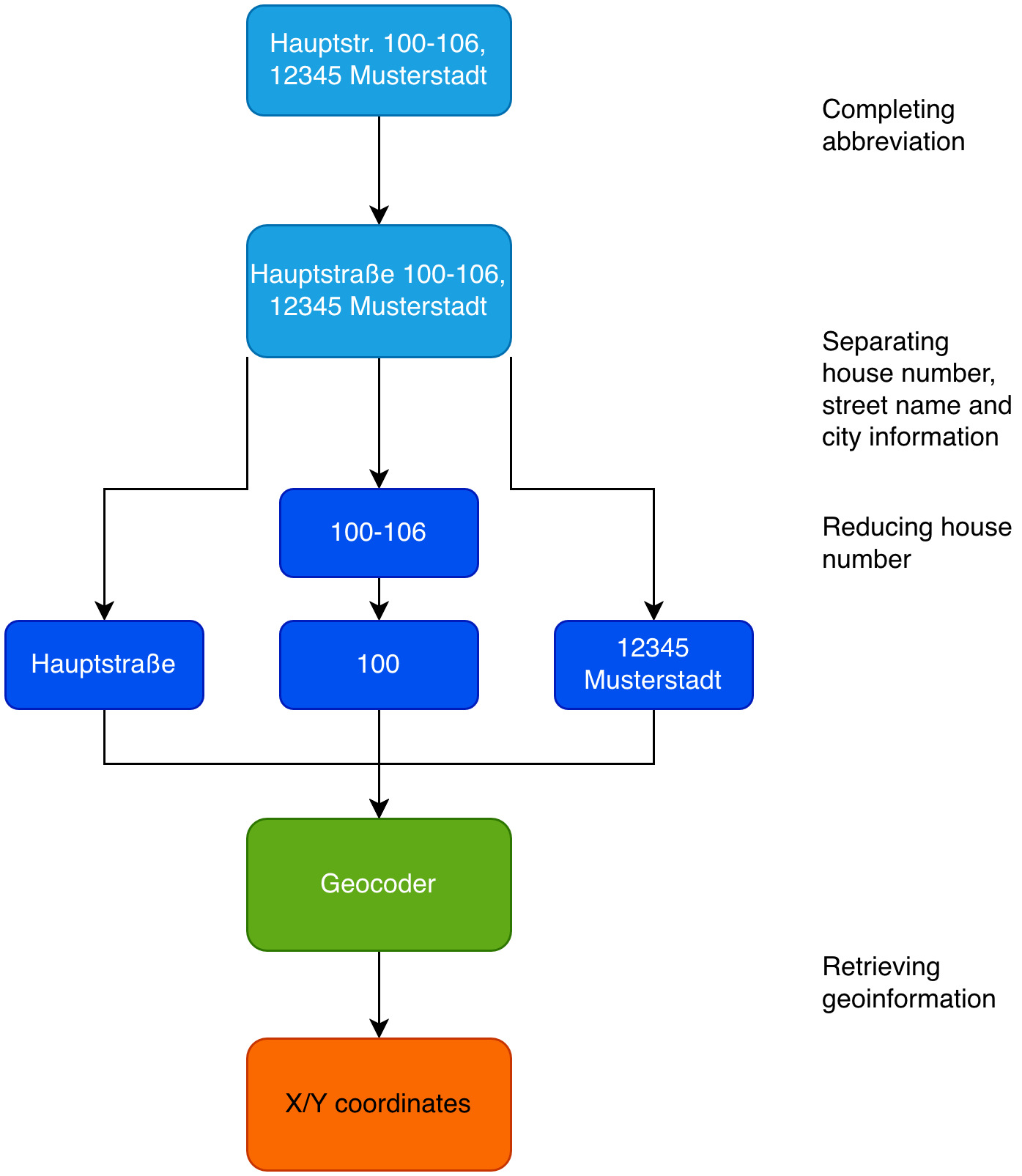
| Second challenge: Address formats spanning multiple house numbers (e.g., “Hauptstraße 100–106”). Standard geocoding tools are often less successful in the case of several house numbers for one address. | To address this, one solution is to use only the first number (e.g., instead of “Hauptstraße 100–106” use “Hauptstraße, 100”). |
| Third challenge: Some addresses require additional protection (such as shelters) to ensure anonymity. | To address this, research ethics require setting those addresses to missing. |
Example of a geocoding workflow
3.2 Example of data quality and coverage
After extensive standardisation:
- Approximately 43 million address records were harmonised.
- Around 19 million geographic coordinates were retrieved.
- Roughly 95% of observations could be linked to exact mailing addresses.
Due to strict data protection regulations, access to geo-referenced administrative data is restricted.
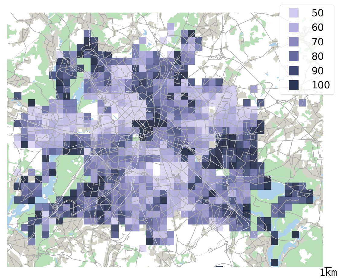
Figure 4 shows, as an example, the inner-city wage distribution across the Berlin city area in 2017. The georeferenced point data was aggregated to 1x1km grid cells. The figure reveals substantive spatial variation in wages. Due to data security reasons, grid cells with fewer than 20 households are not visualized. For more information on the georeferenced administrative data see Ostermann et al. (2022).
4. Geocoded survey data: the example of SOEP
Geodata are also available for survey research. In the German Socio-Economic Panel (SOEP), residential addresses are converted into geographic coordinates under strict confidentiality procedures. The SOEPgeo dataset covers survey waves from 2000 onward and provides longitudinal information, including data for the gross population. However, for confidentiality reasons, researchers do not have simultaneous access to precise coordinates and full panel information.
Figure 5 shows, as an example, the distribution of SOEP respondents across the Berlin city area in 2022. The figure emphasizes the spatial variation in the residential locations of SOEP respondents and highlights the potential of linking these data with grid cell information from different sources. For disclosure control in this visualization, grid cells with fewer than 10 households, in line with census rules, are not shown. In addition, the assignment of observations to grid cells includes a small degree of spatial uncertainty to prevent re-identification. Therefore, fine-scale spatial patterns in the figure should be interpreted with caution.
For scientific purposes, more detailed analyses are possible under controlled conditions: researchers can access the original coordinates at secure on-site facilities of the SOEP Research Data Center (FDZ SOEP). However, even in this setting, no direct linkage to full survey data is permitted. Instead, users may generate and export derived indicators based on external geodata, which can then be merged with the survey data in a separate step.